Gathering the Data
Greg at yhat shows how to scrape the data from Baseball-Reference. Since web scraping makes it easy to grab a lot of data quickly I thought I’d try it. So, I wrote code to scrape game data for all 30 teams through name changes & relocations over the past 25 years, 1990 - 2014. My code for this is in 1-scrapeData.R. It isn’t very pretty, if team names hadn’t changed it would be more succinct. Still, you’ll end up with a file per team, which makes it an easy starting point.
Stadium capacity seems like an important variable, or at least important enough to pursue. Fortunately this data is available on Wikipedia. Unfortunately it isn’t available in a consistent or easily identifiable pattern. I gathered this by searching for each team’s stadium & reading the capacity info. Tedious, but it only took a couple of hours. I included state & stadium name as well. The data for this is contained in data/clean/MLB-Stadium-Capacity.csv.
Cleaning the Data
The data I’ve collected includes one data file per team, and stadium data in a separate file. I create a single data frame for the team data then merge with the stadium data. This is completed in 2-mergeData.R. Now I have ~120k rows of game data that’s formatted for the web. Time to get cleaning.
3-cleaner.R is a single function that cleans or removes each type of data in one pass. I’ve commented what each section does. The function removes variables which I don’t believe will improve predictive ability, removes all away games (these teams are playing each other, so every game is included twice in this data set), and converts every other variable to a format that R can work with.
I will comment on one of the variables that I clean, Date. I convert this to a format that R can work with, then ultimately remove it. I debated removing it altogether and finally chose to leave my code in place so that it’s easy to add this back in for later analysis or visualization.
Some of the variables require more effort than others to clean. It took less than 10 seconds to run on my laptop, and you should end up with a data frame containing 12 columns and ~60k rows of clean data that’s ready for evaluation.
Creating Models
I split the data into train, test & validation sets, then created four models: linear model, decision tree, gradient boosted machine & random forest. I created four models because I wanted to see which would be effective with this particular problem. I chose these four algorithms because they were reasonably easy to run against my data. My work is visible in 4-models.R.
The first three were completed with cross validation (10 folds). This wasn’t necessary with random forests, as a portion of the samples are withheld for testing while the model is being created.
Prediction & Evaluation
I made a prediction using each of my four models (5-predict.R), then calculated the root mean square error and coefficient of determination AKA (R^2) (6-evaluate.R). Normally I would calculate the adjusted (R^2), but since I have rows » variables it isn’t necessary.
| Model | R^2 | RMSE |
|---|---|---|
| lm | 0.472 | 8513.6 |
| dtree | 0.615 | 7264.0 |
| gbm | 0.584 | 7551.0 |
| random forest | 0.728 | 6113.9 |
According to the results, the lineal model performed the worst, with an (R^2) of 0.47. Decision trees and gradient boosted machines were roughly the same, with an (R^2) near 0.6. Random forest was the leader with an (R^2) of 0.73. I’d call that good not great, but its notable that I did very little tuning of these algorithms so this is a good first effort.
Finally I tested my random forest model against the validation set. The results were consistent with the test set.
Next Steps
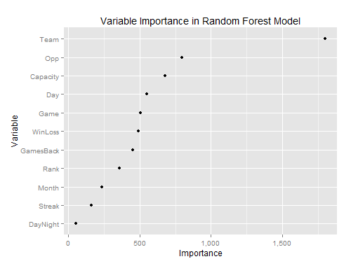
To improve the results of these models, I’d start by evaluating the data again. According to randomForest’s varImpPlot, DayNight is a weak predictor. Maybe replacing that with state or stadium info would help.
Regarding algorithms, I’d start by seeing where I could get with GBM or dtree because they run so much faster. These algorithms took just a few minutes to run, while random forest took several hours. In a production environment, or for final results I may go with random forest, but while trying different sets of variables I’d use GBM or dtree.
The data in its current format has Streak, GamesBack and WinLoss data for the current game (meaning the results of the current game are inclusive in this data). Maybe it would help to shift that so that it reflects the previous game. It would also be pretty simple to show the opponent’s Streak, WinLoss and GamesBack data.
My guess is that Year would be a good predictor as well, but I’ve intentionally excluded it from analysis. I want to be able to predict attendance at all games, including the first few. If I include Year then it will take a few games to train the model for each new season.
These ideas are based on intuition from spending time with the data. I could also get more rigorous and perform principal component analysis on the data prior to creating an algorithm.
As I mentioned earlier, I haven’t tuned my algorithms. Each one has its own set of input parameters. I could spend some time tweaking each. I would start with tuning gradient boosted machines because that algorithm runs much faster than random forests.
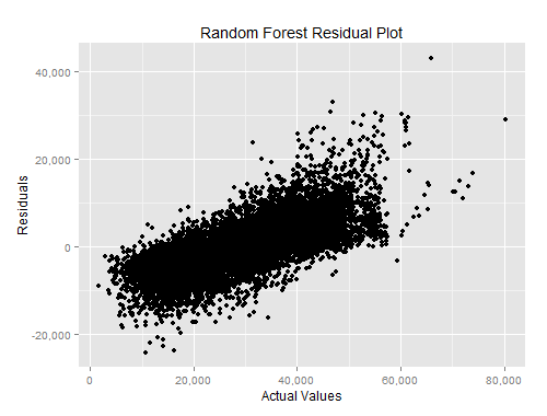
Finally, looking at the residuals plot, my model is less effective for lower and higher attendance games. On either end of the spectrum I have several games that are off by more than 20k. While working with the data I did notice that some games have an attendance higher than stadium capacity. I’m not sure how to deal with this just now, but it probably needs to be accounted for.
I’ll leave these tasks for another look at this data. All of my code for this is available on GitHub.